%load_ext sql
from sqlalchemy import create_engine
%sql postgresql://postgres:****@localhost/dvdrental
engine = create_engine('postgresql://postgres:****@localhost/dvdrental')
Creating indexes is one way to make an execution more efficient, indexes are ordered subsets of data in a table. They can make it more efficient to search for attributes of a certain value. Types of common indexes are:
Indexes can speed up execution time because they reduce the need for full table scans. They can also help to enforce constraints, for example if a column has a unique constraint, before a new value is added to a row, checking if the corresponding value of the index column is already in the index will prompt a constraint conflict. This can be faster than checking the entire table with a full table scan.
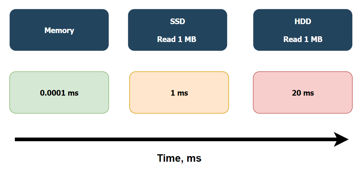
Most of the time, the index is smaller in size than the table. In this case the index is more likely to fit onto the system memory, instead of the solid state drive (SSDs) or hard drive. In this circumstance, the execution time is significantly faster, at around 100 ns, compared to 1 ms or 20 ms for SSDs and hard drives, respectively.
As the name suggests, data in a B-tree index is organised in a tree like structure, with a root and nodes. The root number is roughly the middle value of the dataset, from here the nodes split to the left and to the right of the root. The smaller numbers split to the left and the larger numbers split to the right. This pattern continues until the bottom is reached, the point at which all the data is accounted for.
For example, if the root has a value of 100, the node may split on the left side at 75 and the right side at 125. Each of these nodes will split again, so the left 75 will split to the left at 63 and the right at 87. This pattern continues at each level of the tree, an example of this can be seen below.
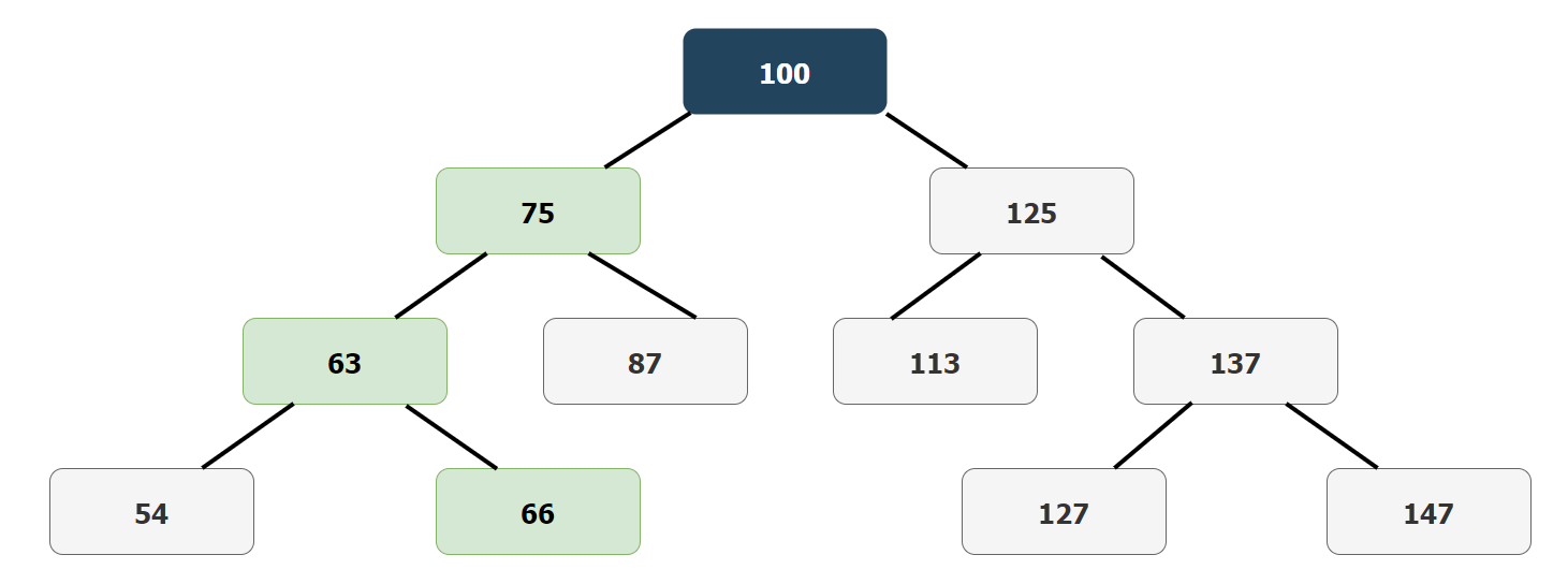
If the value 66 is needed, it would take three comparisons to reach, as seen in the above B-tree index example. From the root at 100 to the left node at 75, then to the left at 63, and finally to the right to reach 66. This path is indicated above in green.
The B-tree index is one of the more common indexes. In PostgreSQL it is the default index. It is useful when there are many uncommon or unique values in a column, which is known as high cardinality.
In the example below, a specific email address is queried from the customer table using the WHERE
statement. At this point there is no index being used. This is known as the query plan states the scan is "Seq Scan", which stands for sequential scan. A sequential scan is the same thing as a full table scan. The computational cost is 16.49
, the planning time is 1.939 ms
and the execution time is 0.142 ms
.
%%sql
EXPLAIN ANALYSE
SELECT *
FROM customer
WHERE email = '[email protected]';
* postgresql://postgres:***@localhost/dvdrental 5 rows affected.
QUERY PLAN |
---|
Seq Scan on customer (cost=0.00..16.49 rows=1 width=70) (actual time=0.026..0.128 rows=1 loops=1) |
Filter: ((email)::text = '[email protected]'::text) |
Rows Removed by Filter: 598 |
Planning Time: 1.939 ms |
Execution Time: 0.142 ms |
The second query below is the same except this time a B-tree index is created called idx_customer_email
on the customer table for the column email
. This is known as the query plan states the scan is an "Index Scan". By using this B-tree index, the overall speed of the query increasing significantly. The computational cost is 8.29
, the planning time is 0.867 ms
and the execution time is 0.048 ms
.
%%sql
CREATE INDEX idx_customer_email ON customer USING btree (email);
EXPLAIN ANALYSE
SELECT *
FROM customer
WHERE email = '[email protected]';
* postgresql://postgres:***@localhost/dvdrental Done. 4 rows affected.
QUERY PLAN |
---|
Index Scan using idx_customer_email on customer (cost=0.28..8.29 rows=1 width=70) (actual time=0.036..0.036 rows=1 loops=1) |
Index Cond: ((email)::text = '[email protected]'::text) |
Planning Time: 0.867 ms |
Execution Time: 0.048 ms |
While B-tree indexes are suited towards high cardinality (many uncommon or unique values in a column) the Bitmap index is more useful for low cardinality columns. A good example of a low cardinality column would be a column which values can only be a "yes" or a "no", there are only 2 options.
Bitmap indexes work by storing a series of bits for each indexed value. The number of bits that are used equals the number of distinct values in the column. Taking the example of the "yes" or "no" column, each value would have 2 bits, one for the "yes" and one for the "no". This example is Boolean, but Bitmap indexes can be used for more than 2 values, when this happens the amount of bits used increases proportionally to the values.
Because Bitmap indexes work especially well on Boolean values, statements such as AND
, OR
and NOT
can run fast compared to other types of indexes.
PostgreSQL creates Bitmap indexes on the fly, so it is possible that a Bitmap index is created without specifically stating this in the query. The following is an example of a Bitmap index in use, this is known as the query plan states the scan is a "Bitmap Heap Scan".
The following two queries observe that both the planning time and the execution time are significantly faster when using the Bitmap index.
%%sql
EXPLAIN ANALYSE
SELECT replacement_cost
FROM film
WHERE replacement_cost = '14.99';
* postgresql://postgres:***@localhost/dvdrental 5 rows affected.
QUERY PLAN |
---|
Seq Scan on film (cost=0.00..66.50 rows=51 width=7) (actual time=0.010..0.404 rows=51 loops=1) |
Filter: (replacement_cost = 14.99) |
Rows Removed by Filter: 949 |
Planning Time: 1.704 ms |
Execution Time: 0.418 ms |
%%sql
CREATE INDEX idx_film_replacement_cost ON film(replacement_cost);
EXPLAIN ANALYSE
SELECT replacement_cost
FROM film
WHERE replacement_cost = '14.99';
* postgresql://postgres:***@localhost/dvdrental Done. 7 rows affected.
QUERY PLAN |
---|
Bitmap Heap Scan on film (cost=4.67..60.77 rows=51 width=7) (actual time=0.037..0.063 rows=51 loops=1) |
Recheck Cond: (replacement_cost = 14.99) |
Heap Blocks: exact=39 |
-> Bitmap Index Scan on idx_film_replacement_cost (cost=0.00..4.66 rows=51 width=0) (actual time=0.032..0.032 rows=51 loops=1) |
Index Cond: (replacement_cost = 14.99) |
Planning Time: 0.660 ms |
Execution Time: 0.083 ms |
The Hash Index uses a hash function. The hash function maps arbitrary length data into string data of a fixed size, the result is a virtually unique hash value. The hash function is designed in such a way that even a slight difference in input can produce a very different hash value output. The exact size of the hash value depends on the algorithm used.
Hash indexes are normally used for equality operations, such as "=", but not for ranges of values. In recent versions of PostgreSQL (10+) the hash index has improved so that it can sometimes take up less memory than B-tree indexes, although the hash index is as fast, but not faster, than a B-tree index. It may be useful to use when the entire query must fit on the system memory.
The following two queries observe that both the planning time and the execution time are significantly faster when using the Hash index.
%%sql
EXPLAIN ANALYSE
SELECT *
FROM address
WHERE district = 'None';
* postgresql://postgres:***@localhost/dvdrental 5 rows affected.
QUERY PLAN |
---|
Seq Scan on address (cost=0.00..15.54 rows=1 width=61) (actual time=0.112..0.113 rows=0 loops=1) |
Filter: ((district)::text = 'None'::text) |
Rows Removed by Filter: 603 |
Planning Time: 1.286 ms |
Execution Time: 0.130 ms |
%%sql
CREATE INDEX idx_address_district ON address USING HASH (district);
EXPLAIN ANALYSE
SELECT *
FROM address
WHERE district = 'None';
* postgresql://postgres:***@localhost/dvdrental Done. 4 rows affected.
QUERY PLAN |
---|
Index Scan using idx_address_district on address (cost=0.00..8.02 rows=1 width=61) (actual time=0.009..0.009 rows=0 loops=1) |
Index Cond: ((district)::text = 'None'::text) |
Planning Time: 0.608 ms |
Execution Time: 0.018 ms |
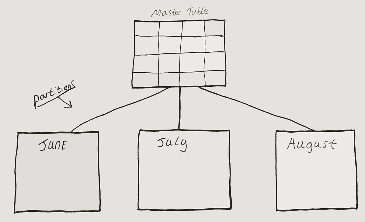
Large tables lead to large indexes. When using a B-tree index for example, the depth of the index grows at an exponential rate to the table size. It is important to be aware of this, but because the index is still much more efficient than a full table scan in most circumstances, this should not be a big problem. With that said, one way around this problem is to partition tables. Table partitioning is a process of separating the table into many smaller tables. This can increase the efficiency of a query because it will run faster on a partition of the table, rather than the whole table. A schematic of this concept is presented below:
This works by using a partition key, which identifies in which partition the rows of interest are stored. One example is to base each partition key on time, one month per partition. Each partition can then also have a local index, to again speed up the execution time of the query. A global index can also be used across all of the partitions, if the filter is not related to the partition key, in this case time.